


MO-210 PDF Exam Material 2026 Realistic MO-210 Dumps Questions
Updated Microsoft MO-210 Dumps – PDF & Online Engine
NEW QUESTION # 11
Instructions
Exam Environment
Exam Interface and Controls
The exam panel provides access to the project task(s). Each project has an associated file in which you will perform the project tasks.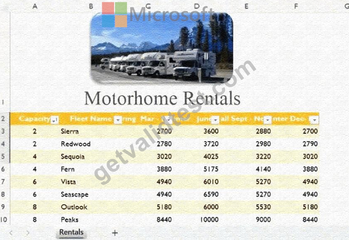
Overview:
Motorhome Rentals
Your company rents motorhomes. The motorhomes rent year-around at different prices. You are preparing pricing worksheets to be shared with others.
Task5:
On the Rentals worksheet, configure the heading row in the table so that entries wider than the column wrap to multiple lines.
Answer:
Explanation:
See the solution in Explanation below.
Explanation:
To ensure that the text in your heading row (the table headers) is fully visible without changing the column width, you will use theWrap Textfeature.
Step-by-Step Solution
* Select the Header Row:In your "Rentals" worksheet, click and drag to select the cell rangeA2:F2(the orange heading row containing "Capacity," "Fleet Name," etc.).
* Navigate to the Home Tab:Ensure you are on theHometab of the Ribbon.
* Apply Wrap Text:
* Look for theAlignmentgroup.
* Click theWrap Textbutton (usually represented by an "ab" icon with a curved arrow).
* Verify the Result:The text in your headers will now automatically wrap to multiple lines if it exceeds the current width of the column.
NEW QUESTION # 12
Instructions
Exam Environment
Exam Interface and Controls
The exam panel provides access to the project task(s). Each project has an associated file in which you will perform the project tasks.
Overview:
Motorhome Rentals
Your company rents motorhomes. The motorhomes rent year-around at different prices. You are preparing pricing worksheets to be shared with others.
Task 4:
Save the Rentals worksheet as a CSV (comma delimited) file named Rentals.csv to the GmetrixTemplates folder.
Answer:
Explanation:
See the solution in Explanation below.
Explanation:
To save a specific worksheet as a CSV file, you need to use theSave Asfunction. This allows you to change the file format from a standard Excel Workbook to a Comma Separated Values file.
Step-by-Step Solution
* Ensure you are currently on theRentalsworksheet (look for the tab name at the bottom of your screen).
* Click theFiletab in the top-left corner.
* SelectSave Asfrom the left-hand menu.
* ClickBrowseto open the File Explorer window.
* In the File Explorer, navigate to theGmetrixTemplatesfolder (usually located in your Documents folder).
* In theFile namebox, typeRentals.
* Click theSave as typedrop-down menu and selectCSV (Comma delimited) (*.csv).
* ClickSave.
* Note:If Excel displays a warning message stating that some features in your workbook might be lost when saving as CSV, clickYesto continue.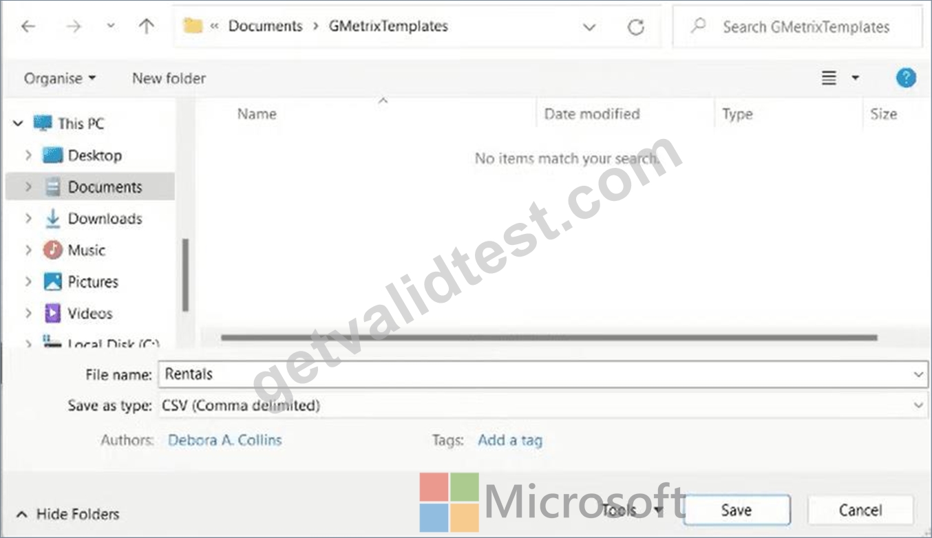
NEW QUESTION # 13
Instructions
Exam Environment
Exam Interface and Controls
The exam panel provides access to the project task(s). Each project has an associated file in which you will perform the project tasks.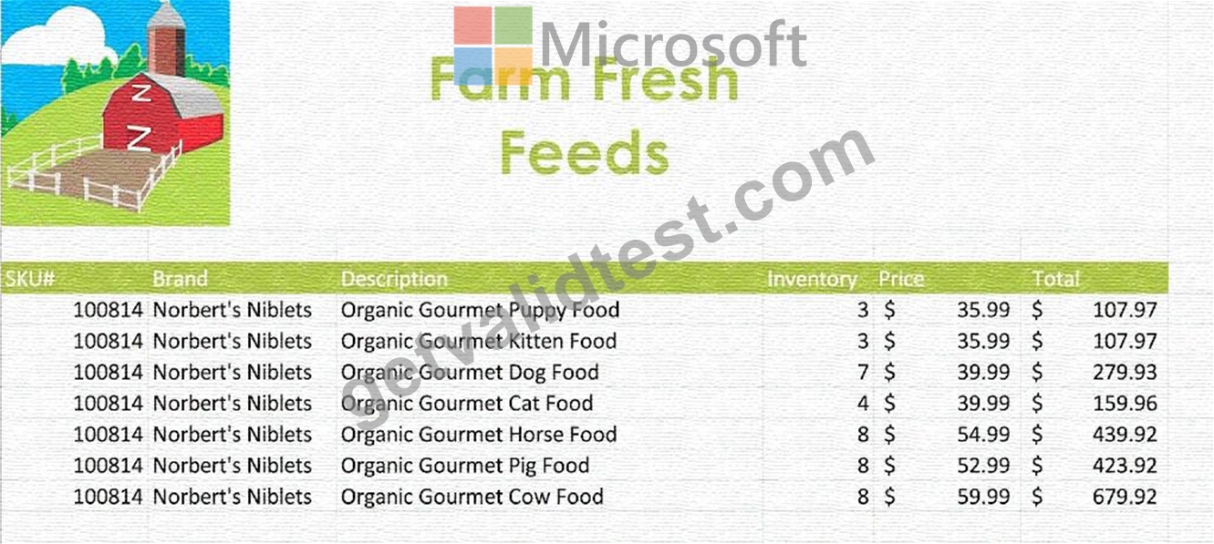
Farm Feeds:
You are the assistant manager for a farm pet feed store. You are creating an inventory report.
Task 2:
Import NewFeeds.txt located in the GMetrixTemplates folder as a table on a new worksheet.
Answer:
Explanation:
See the solution in Explanation below.
Explanation:
To completeTask 2: Import NewFeeds.txt as a table on a new worksheet, follow these exact steps in Microsoft Excel 365:
Step 1: Open the Import Tool
* Go to theDatatab on the top Ribbon.
* In theGet & Transform Datagroup, click onFrom Text/CSV.
Step 2: Locate the File
* A file browser window will open. Navigate to theGMetrixTemplatesfolder.
* Select the file namedNewFeeds.txt.
* ClickImport.
Step 3: Configure the Import Preview
* A preview window will appear. Excel should automatically detect the delimiter (usually a tab or comma).
* Ensure theFile OriginandDelimiterlook correct in the preview.
* Instead of clicking "Load," click thearrow next to the Load buttonand selectLoad To....
Step 4: Import as a Table on a New Worksheet
* In theImport Datadialog box that appears, select the radio button forTable.
* Under "Where do you want to put the data?", selectNew worksheet.
* ClickOK.
Final Result
Excel will create a brand new sheet (e.g., "Sheet2") and place the contents of NewFeeds.txt inside a formatted Excel Table.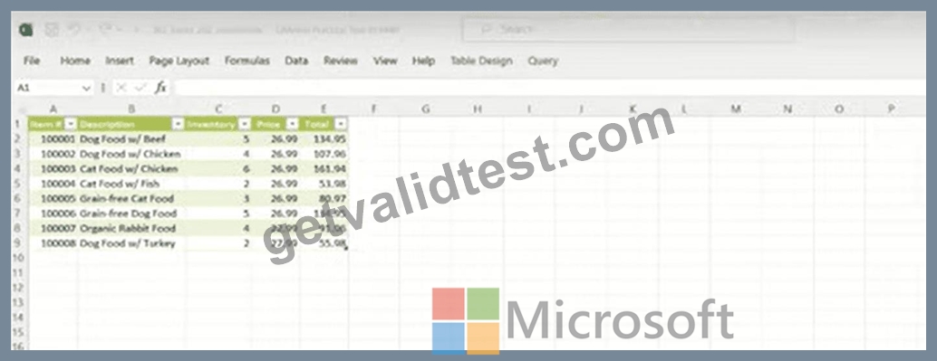
NEW QUESTION # 14
Instructions
Exam Environment
Exam Interface and Controls
The exam panel provides access to the project task(s). Each project has an associated file in which you will perform the project tasks.
Project 1
Overview:
Video Games
You are tracking video game popularity by compiling a workbook to document your findings.
Task 2:
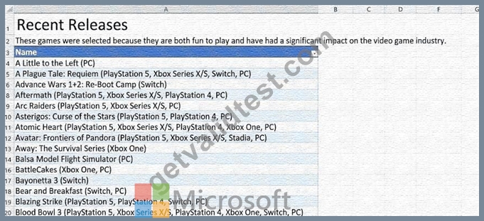
On the Top 20 Videos worksheet, change the width of column C to 2.
Answer:
Explanation:
Here are the complete solutions below.
Explanation:
Step-by-Step Instructions
* Navigate to the Correct Worksheet:
* Click on the tab labeled Top 20 Videos at the bottom of the Excel window to ensure you are on the correct sheet.
* Select Column C:
* Click on the letter C in the column header to select the entire column.
* Open Column Width Settings:
* Method A (Ribbon): Go to the Home tab. In the Cells group (towards the right), click Format.
Select Column Width... from the dropdown menu.
* Method B (Right-click): Right-click directly on the column header "C". A context menu will appear. Click Column Width...
* Enter the Width:
* A small dialog box labeled "Column Width" will appear.
* Type 2 in the box.
* Click OK.
Visual Verification
Before: Column C (containing the "Year" data) is likely wider, fitting the four-digit years comfortably.
After: Column C will become very narrow. The "Year" header and the dates (like 2011, 1984) might display as hashes (####) because the column is now too narrow to display the numbers, or the text will simply be cut off. This is expected behavior for the exam task; do not widen it back out unless instructed to do so.
NEW QUESTION # 15
Instructions
Exam Environment
Exam Interface and Controls
The exam panel provides access to the project task(s). Each project has an associated file in which you will perform the project tasks.
Overview:
Motorhome Rentals
Your company rents motorhomes. The motorhomes rent year-around at different prices. You are preparing pricing worksheets to be shared with others.
Task 3:
Set cells A1:F11 so they will be the only cells that print.
Answer:
Explanation:
See the solution in Explanation below.
Explanation:
To ensure that only a specific range of cells is printed, you need to define aPrint Area. This prevents Excel from printing empty pages or extra data outside of your selection.
Step-by-Step Solution
* Select the range:Use your mouse to click on cellA1and drag your cursor down to cellF11to highlight the entire area.
* Navigate to Page Layout:Click on thePage Layouttab in the top Ribbon.
* Set the Print Area:
* Locate thePage Setupgroup.
* Click on thePrint Areabutton.
* From the drop-down menu, selectSet Print Area.
Once this is set, Excel will only print the content within A1:F11, even if there is data elsewhere on the sheet.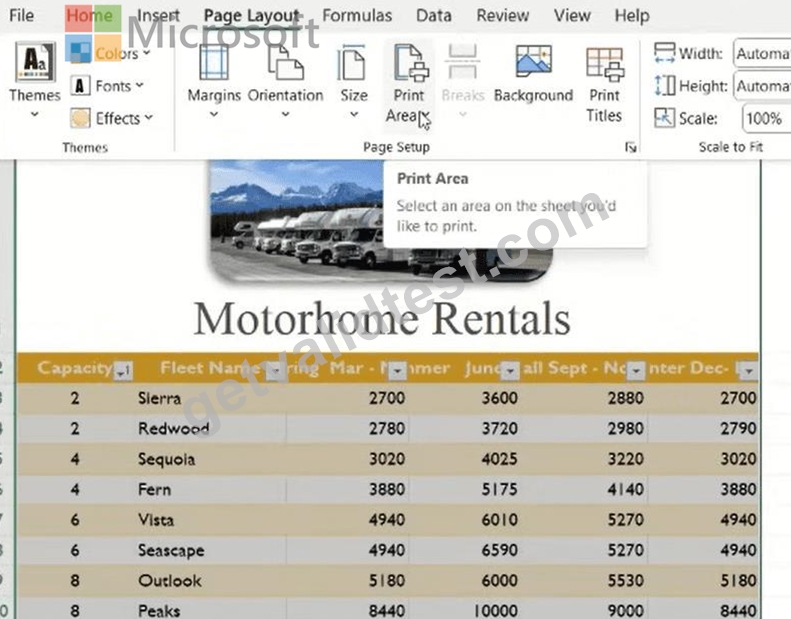
NEW QUESTION # 16
Instructions
Exam Environment
Exam Interface and Controls
The exam panel provides access to the project task(s). Each project has an associated file in which you will perform the project tasks.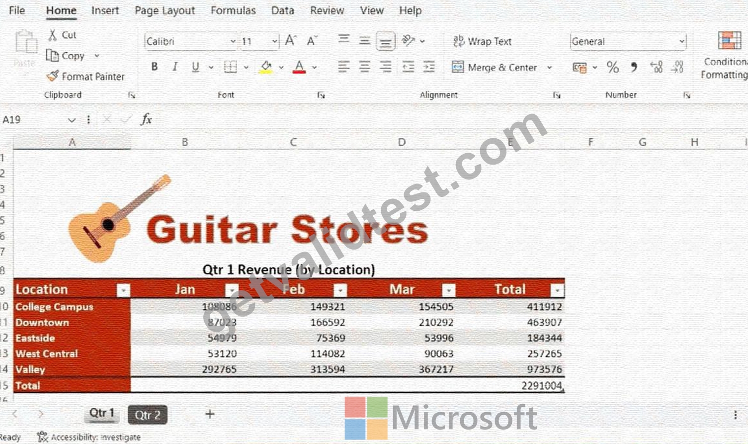
Overview:
Guitar Stores
You and a partner own several Guitar Stores. You are analyzing your revenue from the past two quarters.
Task5:
Display the formulas that are in the cells of the Qtr 2 worksheet.
Answer:
Explanation:
See the solution in Explanation below.
Explanation:
To display the formulas within the cells of the Qtr 2 worksheet instead of the resulting values, you can use the Show Formulas command.
Step 1: Navigate to the Qtr 2 Worksheet
Open your Excel workbook.
Click on the Qtr 2 sheet tab at the bottom of the screen.
Step 2: Enable "Show Formulas" via the Ribbon
Go to the Formulas tab on the Ribbon at the top of the Excel window.
Locate the Formula Auditing group.
Click the Show Formulas button.
Alternative Method: Keyboard Shortcut
You can quickly toggle this view on and off by pressing:
Ctrl + ` (the accent mark or backtick key, usually located to the left of the "1" key).
What to Expect
Once activated, Excel will:
Expand column widths to accommodate the formula text.
Hide the calculated results and show the actual syntax (e.g., instead of seeing $411,912, you will see =SUM (B10:D10)).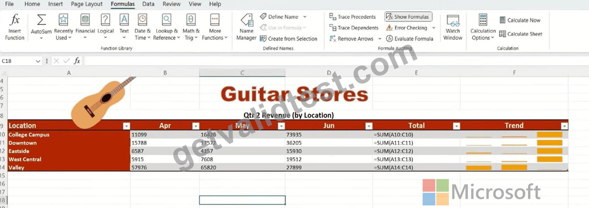
NEW QUESTION # 17
Instructions
Exam Environment
Exam Interface and Controls
The exam panel provides access to the project task(s). Each project has an associated file in which you will perform the project tasks.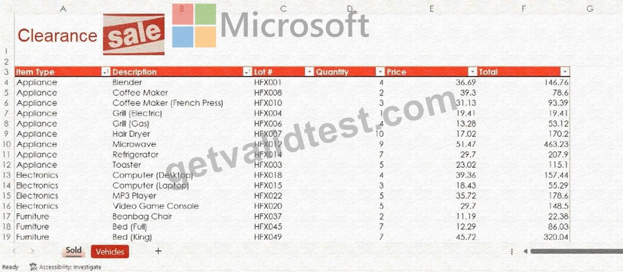
Overview:
Clearance Sale
You are the administrative assistant for a retail company that is going out of business. You've been tasked to prepare a workbook for the clearance sale.
Task 2:
Open a second window and view the two instances of the workbook side-by-side.
Answer:
Explanation:
See the solution in Explanation below.
Explanation:
To view two instances of your Excel workbook side-by-side, follow these steps:
Step 1: Open a Second Window
* Go to theViewtab on the Ribbon.
* In theWindowgroup, click onNew Window.
* Note: This creates a second view of your current file. You will notice the file name in the title bar now says "Filename - 2".
Step 2: Arrange Side-by-Side
* Navigate back to theViewtab.
* In the sameWindowgroup, click theView Side by Sidebutton.
* If the windows do not align automatically, clickArrange Alland selectVerticalto see them left-to-right.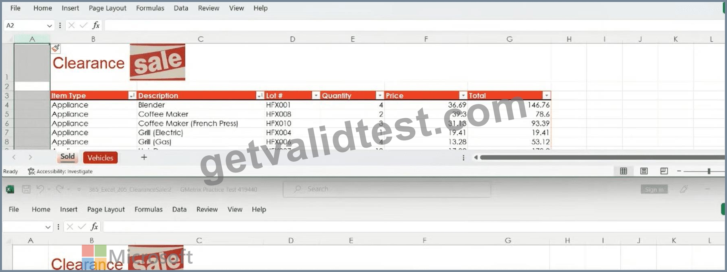
Verification
You should now see two separate windows of the same "Clearance Sale" workbook on your screen. Any change you make in one window will instantly update in the other, allowing you to view different worksheets (like "Sold" and "Vehicles") at the same time.
NEW QUESTION # 18
Instructions
Exam Environment
Exam Interface and Controls
The exam panel provides access to the project task(s). Each project has an associated file in which you will perform the project tasks.
Project 1
Overview:
Video Games
You are tracking video game popularity by compiling a workbook to document your findings.
Task 1:
On the Recent Releases worksheet, select all of the video game titles in the cell range named No Platform and delete their rows. Retain all other cells on the worksheet.
Answer:
Explanation:
Here are the complete solutions below.
Explanation:
Step-by-Step Instructions (Text Only)
Step 1: Activate the correct worksheet
* Open the Excel workbook provided for the project.
* At the bottom of the workbook, click the Recent Releases worksheet tab to make it active.
Step 2: Select the named range "No Platform"
* Click anywhere inside the worksheet.
* Go to the Formulas tab on the Excel ribbon.
* In the Defined Names group, click Name Manager.
* In the Name Manager dialog box:
* Locate the named range called No Platform.
* Click No Platform to select it.
* Click Close.
* Excel will automatically highlight all cells included in the No Platform named range.
(Alternative method if allowed)
* Click the Name Box (left of the formula bar), type No Platform, and press Enter.
Step 3: Select entire rows for the named range
* With the No Platform cells selected:
* Move the cursor to the row numbers on the left side of the worksheet.
* Click the row number of one selected cell.
* Hold down the Ctrl key.
* Click each additional row number that corresponds to the selected No Platform cells until all required rows are selected.
Step 4: Delete the selected rows
* Go to the Home tab on the ribbon.
* In the Cells group, click the Delete drop-down arrow.
* Select Delete Sheet Rows.
Step 5: Verify the result
* Confirm that:
* All video game titles that had no platform information are removed.
* All remaining rows and worksheet content are intact.
* Ensure no extra cells, columns, or headers were deleted.
Final Result
* All rows associated with the No Platform named range are deleted.
* All other data on the Recent Releases worksheet remains unchanged.
* Task 1 is completed correctly according to Excel 365 simulation requirements.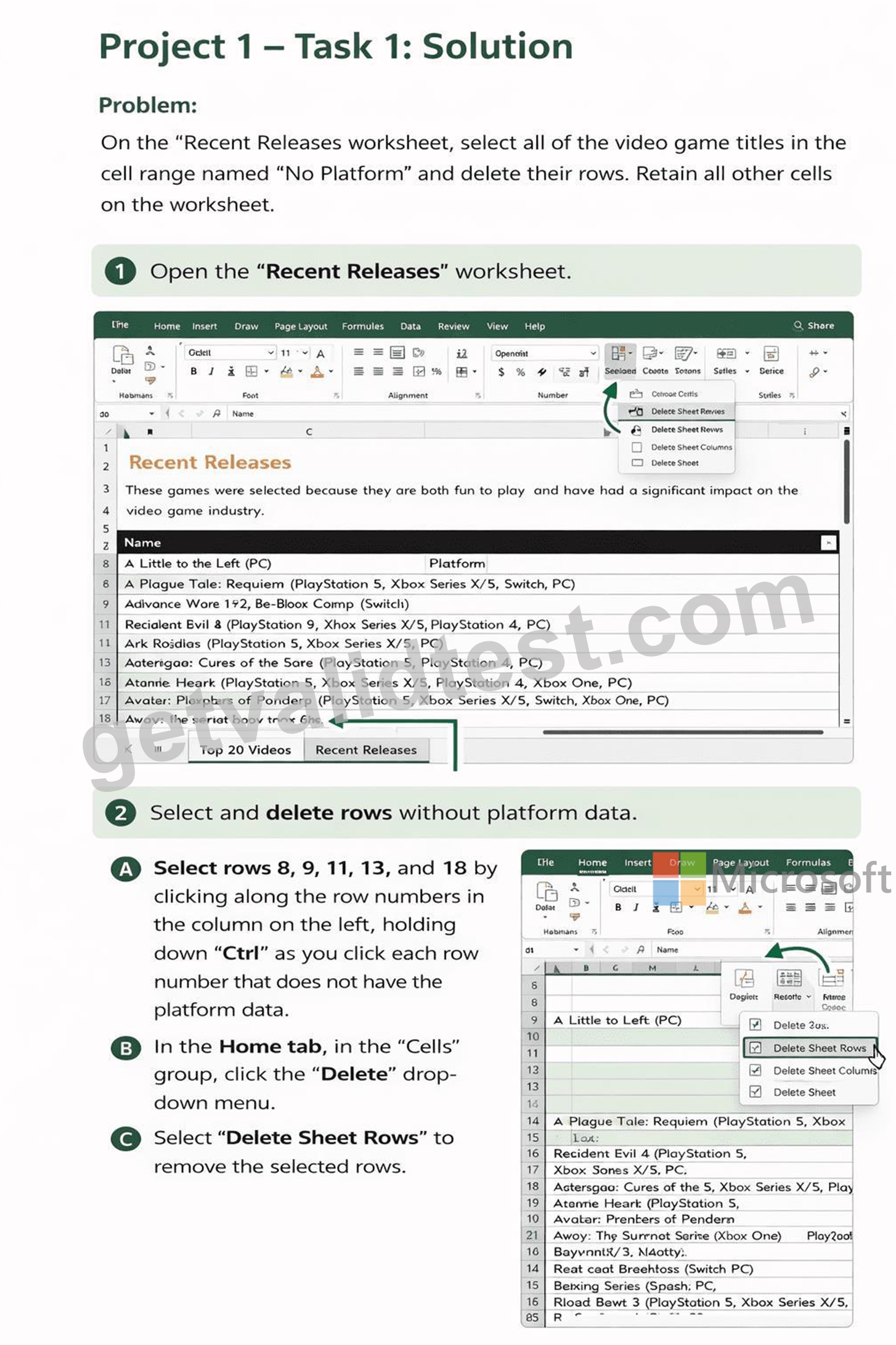
NEW QUESTION # 19
Instructions
Exam Environment
Exam Interface and Controls
The exam panel provides access to the project task(s). Each project has an associated file in which you will perform the project tasks.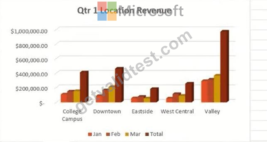
Overview:
Guitar Stores
You and a partner own several Guitar Stores. You are analyzing your revenue from the past two quarters.
Task 1:
In the Qtr 1 worksheet change the configuration of the Q1 Location Revenue chart so that it displays the months on the x-axis and the revenue on they-axis.
Answer:
Explanation:
See the solution in Explanation below.
Explanation:
To swap the data on the axes so that the months appear on the x-axis and the revenue values appear on the y- axis, you will use theSwitch Row/Columnfeature in Excel.
Step 1: Select the Chart
* Go to theQtr 1worksheet.
* Click once on the border of theQ1 Location Revenuechart to select it. This will reveal theChart Design andFormattabs on the Ribbon.
Step 2: Switch Row/Column Data
* With the chart selected, click on theChart Designtab at the top of the window.
* Locate theDatagroup on the right side of the Ribbon.
* Click theSwitch Row/Columnbutton.
Step 3: Verify the Change
* The X-Axis (Horizontal):Should now display the month labels (Jan, Feb, Mar).
* The Legend:Should now display the differentLocations(College Campus, Downtown, etc.) as the colored series.
* The Y-Axis (Vertical):Will automatically scale to represent the revenue values.
NEW QUESTION # 20
Instructions
Exam Environment
Exam Interface and Controls
The exam panel provides access to the project task(s). Each project has an associated file in which you will perform the project tasks.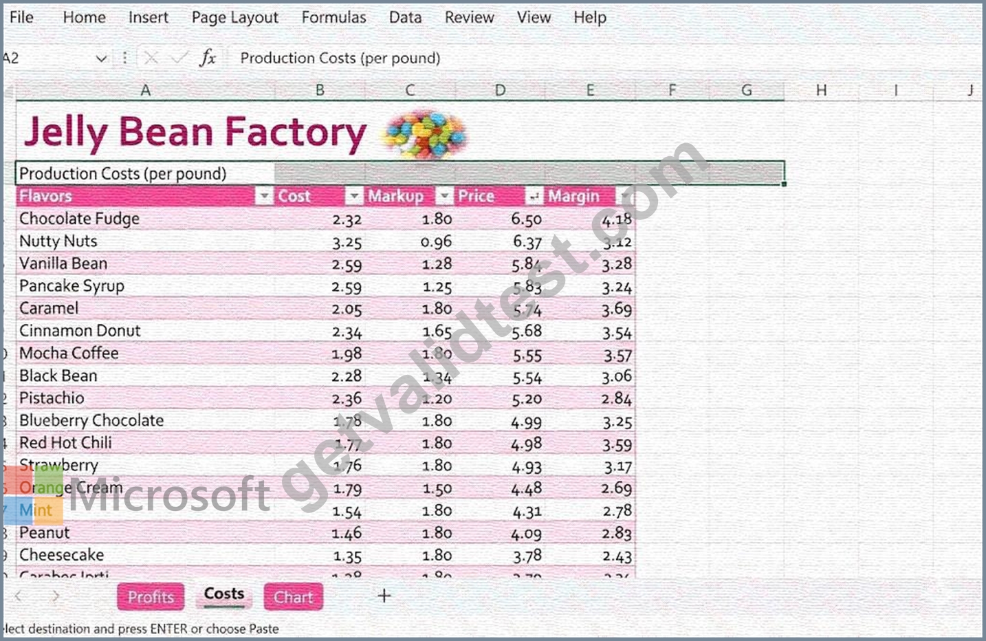
Overview:
Jelly Beans
A shop you manage sells gourmet jelly beans. You are tracking the amount of jelly beans sold each quarter and summarizing the information in aworkbook.
Task 5:
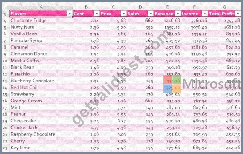
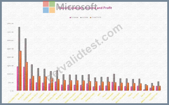
Group the Profits, Costs, and Chart worksheets and change the tab color to Pink, Accent 4.
Answer:
Explanation:
See the solution in Explanation below.
Explanation:
To group multiple worksheets and change their tab colors simultaneously in Microsoft Excel 365, follow these steps:
Step 1: Group the Worksheets
* Look at the worksheet tabs at the bottom of your Excel window.
* Click on the first tab,Profits.
* Hold down theCtrlkey on your keyboard.
* While holdingCtrl, click on theCoststab and then theCharttab.
* Note: You will notice all three tabs now have a white background, indicating they are grouped together.
Step 2: Change the Tab Color
* Right-clickon any of the selected (grouped) tabs.
* Hover your mouse overTab Colorin the pop-up menu.
* In the color palette that appears, locate theTheme Colorssection.
* Find and selectPink, Accent 4(this is usually the 8th color in the top row of the Theme Colors section).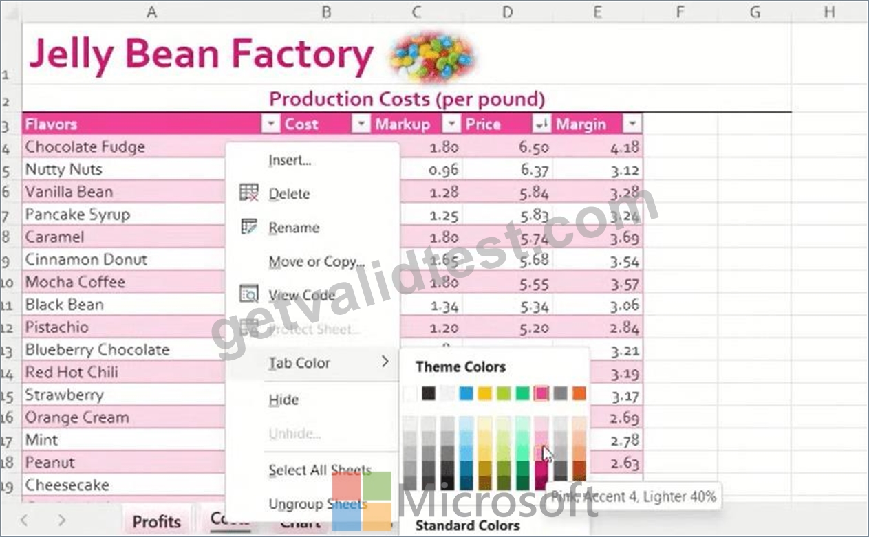
Step 3: Ungroup the Worksheets
* To finish,right-clickon any of the tabs again.
* SelectUngroup Sheetsfrom the menu.
* Alternatively, you can click on any worksheet tab that is not part of the group to ungroup them.
Final Result
TheProfits,Costs, andCharttabs will now all display the samePink, Accent 4color at the bottom of your workbook.
Would you like me to help you with the next task or another project?
NEW QUESTION # 21
Instructions
Exam Environment
Exam Interface and Controls
The exam panel provides access to the project task(s). Each project has an associated file in which you will perform the project tasks.
Farm Feeds:
You are the assistant manager for a farm pet feed store. You are creating an inventory report.
Task 1:
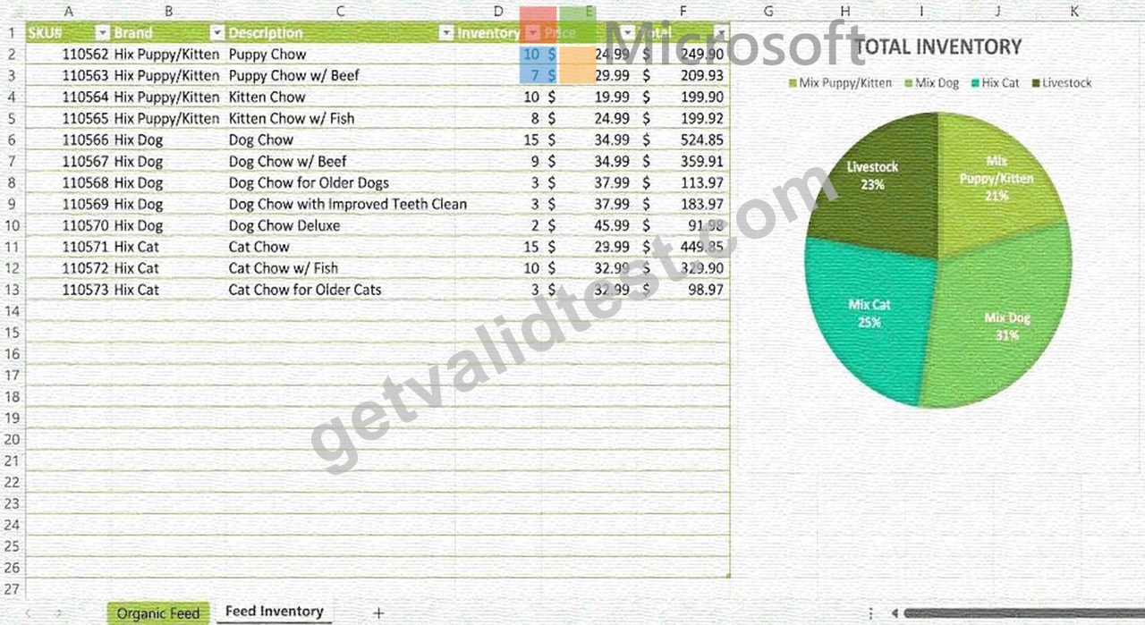
Remove the conditional formatting from the table on on the Feed Inventory worksheet.
Answer:
Explanation:
See the solution in Explanation below.
Explanation:
To completeTask 1: Remove the conditional formatting from the table on the Feed Inventory worksheet
, follow these steps:
Step 1: Select the Target Worksheet
First, ensure you are on the correct worksheet as specified in the instructions.
* Click on theFeed Inventorytab at the bottom of your Excel workbook.
Step 2: Select the Table or Data Range
You can remove formatting from the entire sheet, but to be precise with the "table," follow these sub-steps:
* Click anywhere inside the table (the area containing the SKU#, Brand, Description, etc.).
* PressCtrl + Ato select the entire table range.
Step 3: Access the Conditional Formatting Menu
* Go to theHometab on the top Ribbon.
* In theStylesgroup, click on theConditional Formattingbutton.
Step 4: Clear the Rules
* Hover your mouse overClear Rulesnear the bottom of the drop-down menu.
* A side menu will appear. SelectClear Rules from Selected Cells(if you have the table selected) or Clear Rules from Entire Sheetto ensure all formatting is removed.
Final Result
Once clicked, any data bars, color scales, or highlight rules (like the light green shading seen in your screenshot) that were applied via Conditional Formatting will be removed, leaving the standard table styling
NEW QUESTION # 22
Instructions
Exam Environment
Exam Interface and Controls
The exam panel provides access to the project task(s). Each project has an associated file in which you will perform the project tasks.
Overview:
Guitar Stores
You and a partner own several Guitar Stores. You are analyzing your revenue from the past two quarters.
Task 1:
On the Qtr 2 worksheet, in cell F10, insert a column sparkline showing the sales trend from Apr through Jun.
Apply Gold, Sparkline Style Accent 2,Darker 25% to the sparkline. Copy the sparkline to the remaining cells in the column, F11:F14.
Answer:
Explanation:
See the solution in Explanation below.
Explanation:
here is the step-by-step solution for Task 1:
Step 1: Navigate to the Correct Worksheet
Click on theQtr 2worksheet tab at the bottom of the Excel window to ensure you are working on the correct data set.
Step 2: Insert the Column Sparkline
* Click on cellF10(this is where the first sparkline will reside).
* Go to theInserttab on the Ribbon.
* In theSparklinesgroup, click onColumn.
* A dialog box will appear. ForData Range, select the cells representingApr through Junfor the first row (likelyB10:D10).
* Ensure theLocation Rangeis set to$F$10.
* ClickOK.
Step 3: Apply the Specific Sparkline Style
With cellF10still selected, a newSparklinetab will appear at the top of your Ribbon.
* Click on theSparklinetab.
* Click theMorearrow (the small downward arrow at the bottom right) of theStylesgallery to see all options.
* Hover over the styles to find the specific name:Gold, Sparkline Style Accent 2, Darker 25%.
* Click to apply it.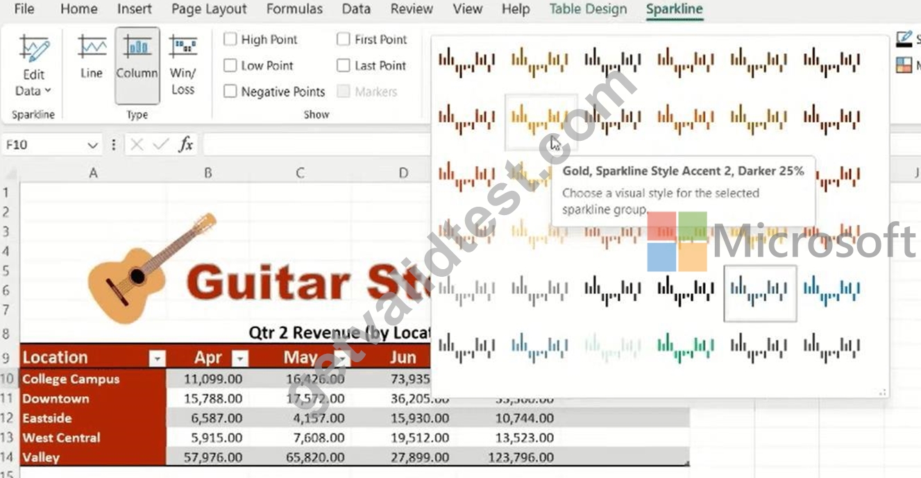
Step 4: Copy the Sparkline to Remaining Cells
* Select cellF10.
* Hover your mouse over theFill Handle(the small green square in the bottom-right corner of the cell).
* Click and drag the handle down to cellF14.
* Excel will automatically generate sparklines for the other locations (Downtown, Eastside, etc.) using the same style and corresponding data rows.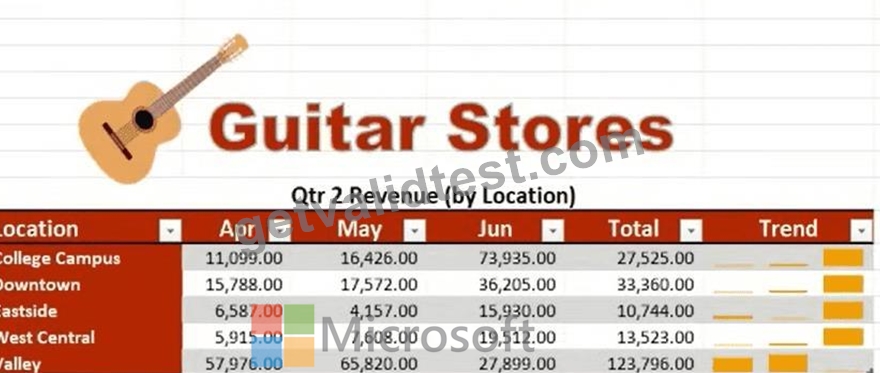
NEW QUESTION # 23
Instructions
Exam Environment
Exam Interface and Controls
The exam panel provides access to the project task(s). Each project has an associated file in which you will perform the project tasks.
Farm Feeds:
You are the assistant manager for a farm pet feed store. You are creating an inventory report.
Task 3:
On the Feed Inventory worksheet, remove the hyperlink functionality, but leave the text in cell C27.
Answer:
Explanation:
See the solution in Explanation below.
Explanation:
To completeTask 3: Remove the hyperlink functionality from cell C27 on the Feed Inventory worksheet, follow these specific steps to ensure the text remains while the link is deleted.
Step 1: Select the "Feed Inventory" Worksheet
Ensure you are on the correct sheet by clicking theFeed Inventorytab at the bottom of the window.
Step 2: Navigate to Cell C27
Locate cellC27in the Description column. Based on your project files, this is likely a URL or a linked piece of text at the bottom of the table.
Step 3: Remove the Hyperlink
You want to strip the "clickable" link without deleting the actual words inside the cell.
* Right-clickdirectly on cellC27.
* From the context menu that appears, selectRemove Hyperlink(it is usually located at the very bottom of the list).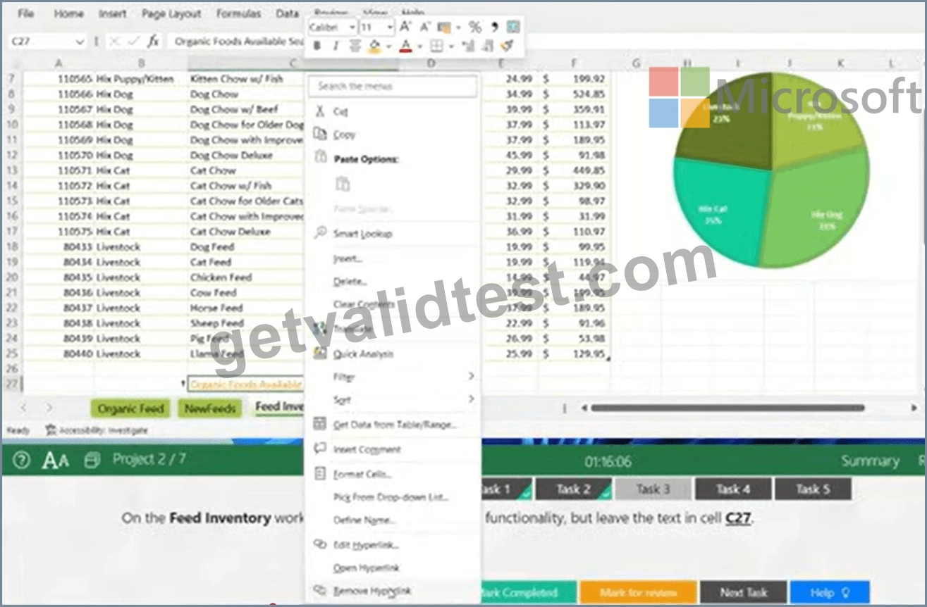
Step 4: Verify the Text Remains
The text should change from blue/underlined back to standard black text, but the characters themselves will stay in the cell.
NEW QUESTION # 24
Instructions
Exam Environment
Exam Interface and Controls
The exam panel provides access to the project task(s). Each project has an associated file in which you will perform the project tasks.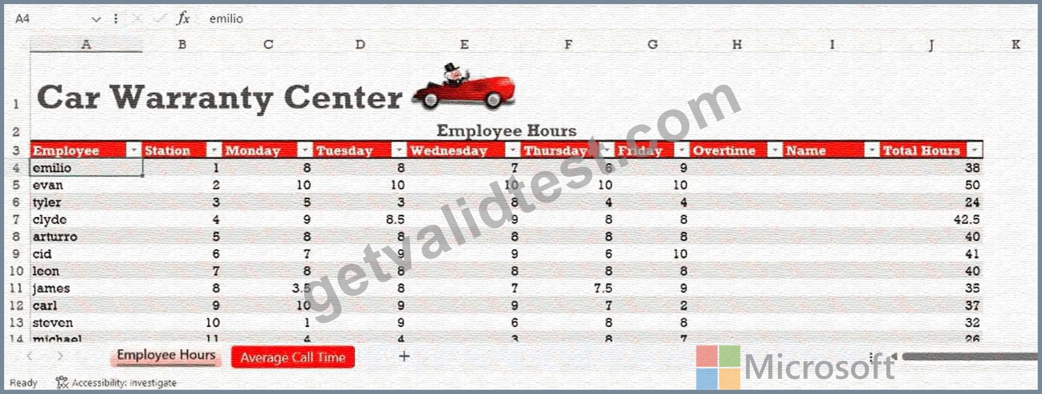
Overview:
Car Warranty
You are the supervisor for a Car Warranty Center. You use Excel to report employee hours and telephone calls.
Task 1:
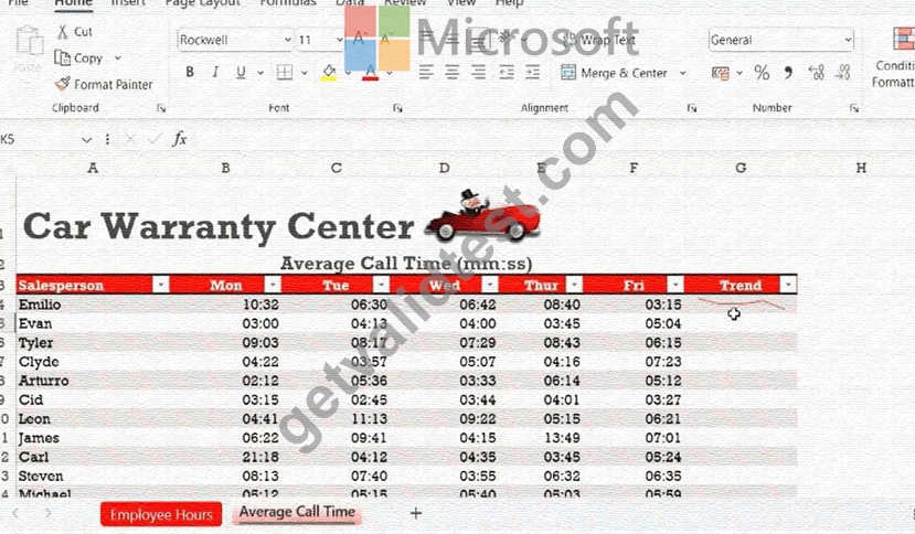
On the Average Call Time worksheet, use an Excel feature to copy the sparkline into all the vacant cells of the Trend column.
Answer:
Explanation:
See the solution in Explanation below.
Explanation:
n Excel 365, the most efficient way to do this is using theAutoFillfeature or simply dragging the fill handle.
Here is your step-by-step solution:
Step 1: Switch to the Correct Worksheet
Ensure you are on theAverage Call Timeworksheet. Click the red tab at the bottom of the screen to switch from the "Employee Hours" view (shown in your image) to the call time data.
Step 2: Identify the Sparkline
Locate the first cell in theTrendcolumn that already contains a Sparkline (likely cellF4or similar, depending on your layout).
Step 3: Use the Fill Handle to Copy
* Hover your mouse over thebottom-right cornerof the cell containing the sparkline.
* Your cursor will change from a thick white cross to athin black cross (+).
* Click and dragthe fill handle down to the bottom of the column to fill all the vacant cells in the
"Trend" column.
Pro Tip:Alternatively, you can simplydouble-clickthe thin black cross (fill handle), and Excel will automatically fill the sparklines down to the last row of your data.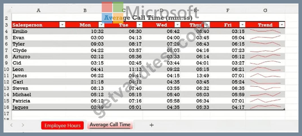
Alternative Method: Using the Ribbon
If you prefer using the menu interface:
* Select the cellwith the existing sparkline and all theempty cells below itwhere you want the sparklines to appear.
* Go to theHometab.
* In theEditinggroup, click theFillicon (downward arrow).
* SelectDown.
NEW QUESTION # 25
......
Microsoft MO-210 Dumps PDF Are going to be The Best Score: https://www.getvalidtest.com/MO-210-exam.html
MO-210.pdf - Questions Answers PDF Sample Questions Reliable: https://drive.google.com/open?id=1sCSNt5Bxlr02JophpSNzd9TTuP5eAnuX